DiffusionPDE: Generative PDE-Solving
Under Partial Observation

NeurIPS 2024 ICML 2024 AI for Science Workshop Oral

1University of Michigan 2Stanford University

2.5%
forward error on Darcy Flow, vs. 28–49% for baselines
3%
sparse observation points per scene
5
PDE families, from Darcy Flow to Navier–Stokes

TL;DR DiffusionPDE solves forward and inverse PDEs from partial observations using diffusion models. It learns the joint distribution of a PDE’s inputs and outputs, then recovers both from sparse observations, guided by the observations and the PDE itself.

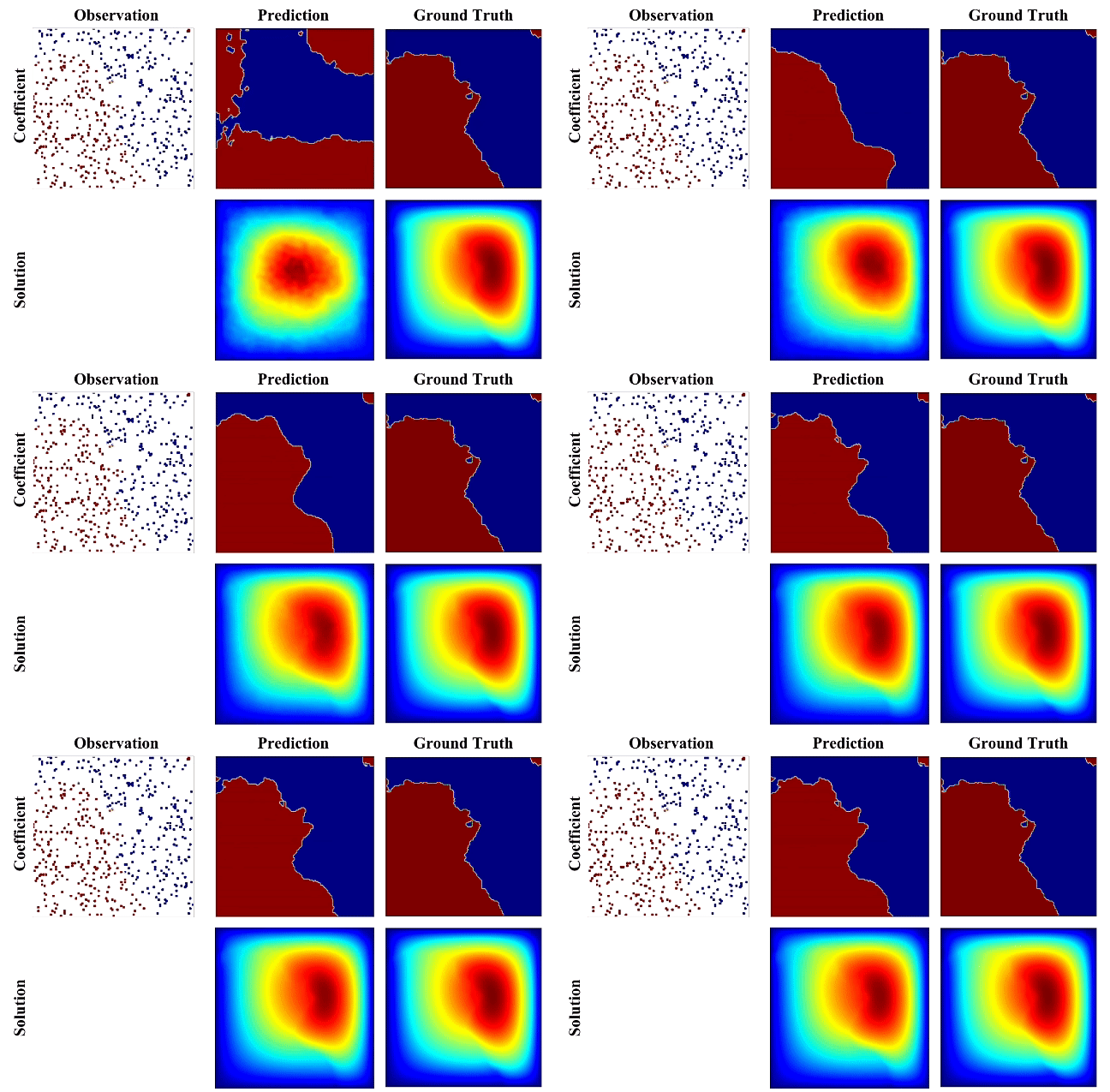
Denoising process for Darcy Flow, guided by sparse observations of the coefficient
Darcy Flow
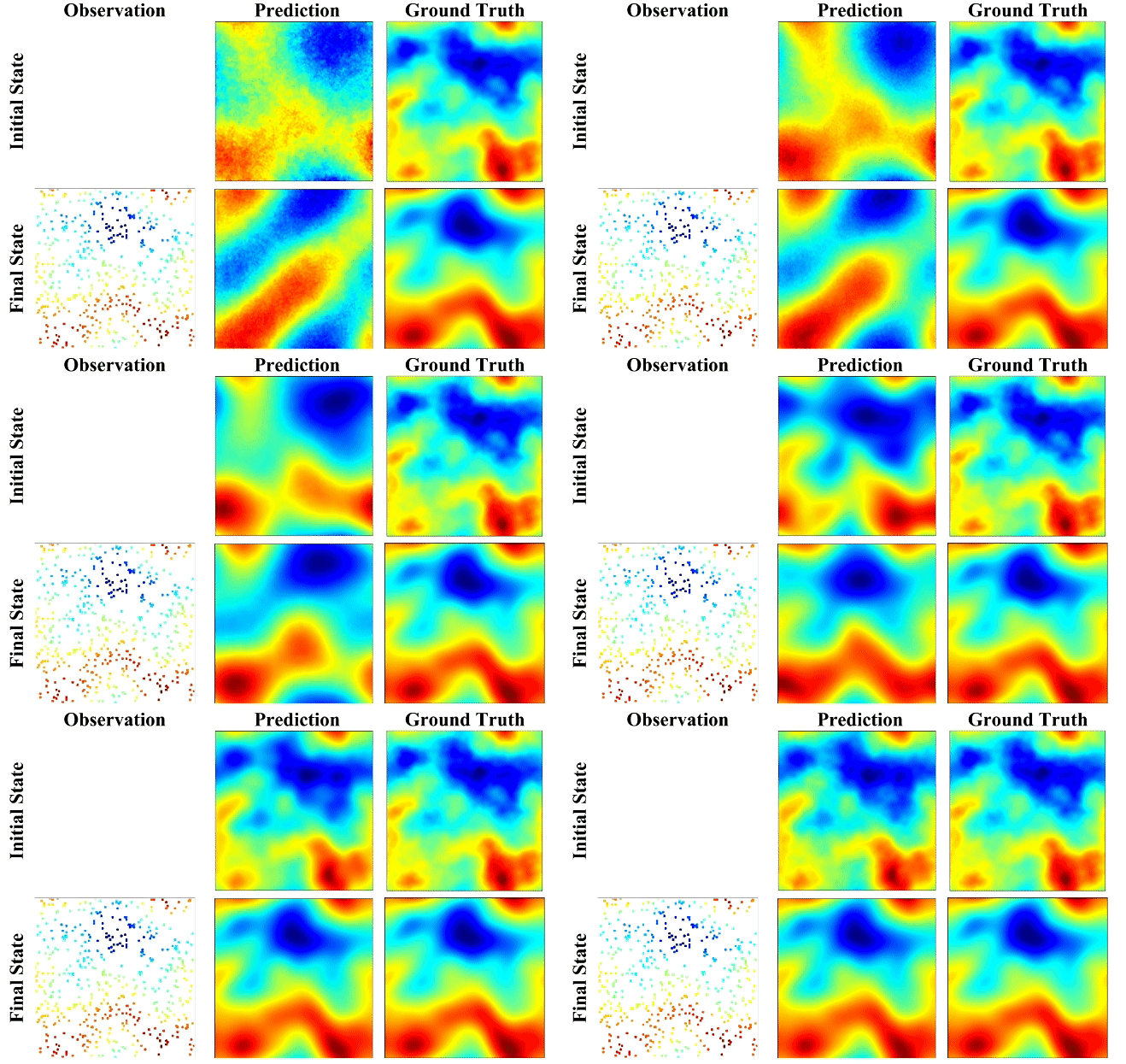
Denoising process for Navier-Stokes vorticity, guided by sparse observations of the final state
Navier–Stokes (vorticity)

Denoising Darcy Flow (left) and the Navier–Stokes equation for vorticity (right) with observations of the coefficient or the final state.

Abstract

We introduce DiffusionPDE, a general framework for solving partial differential equations (PDEs) using generative diffusion models. In particular, we focus on the scenarios where we do not have the full knowledge of the scene necessary to apply classical solvers. Most existing forward or inverse PDE approaches perform poorly when the observations on the data or the underlying coefficients are incomplete, which is a common assumption for real-world measurements. In this work, we propose DiffusionPDE that can simultaneously fill in the missing information and solve a PDE by modeling the joint distribution of the solution and coefficient spaces. We show that the learned generative priors lead to a versatile framework for accurately solving a wide range of PDEs under partial observation, significantly outperforming the state-of-the-art methods for both forward and inverse directions.


Method

Method Overview

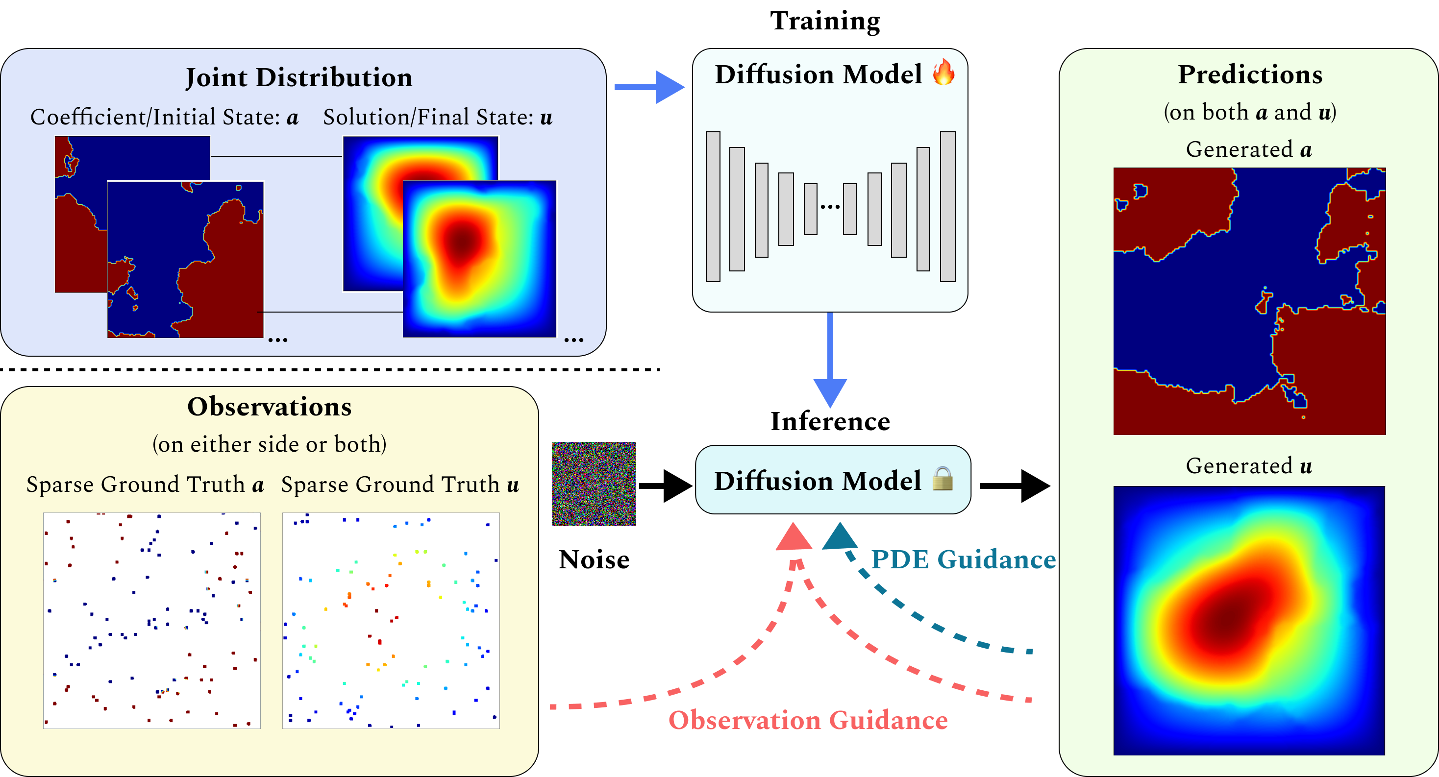
DiffusionPDE overview: a diffusion model trained on the joint distribution of coefficients and solutions, guided at inference by sparse observations and the PDE
Overview of DiffusionPDE. Click any figure to enlarge.
  1. Learn the joint distribution

    Train a diffusion model on full coefficient (or initial state) and solution (or final state) pairs, concatenated along channels.

  2. Observe sparsely

    At inference, only sparse points are known on the coefficient side, the solution side, or both.

  3. Guide the sampling

    Observation guidance and PDE guidance steer the pre-trained model to complete predictions of both sides.

In our framework, we train a diffusion model on the joint distribution of the complete observations of the coefficient (or initial state) and the solution (or final state), concatenated along the channel dimension. During inference, sparse observations are made on either the coefficient (or initial state) side, the solution (or final state) side, or both. The pre-trained model is then guided by these sparse observations and the PDE function to output the final full predictions of both the coefficient (or initial state) and the solution (or final state).


Results

Solving Forward and Inverse Problems

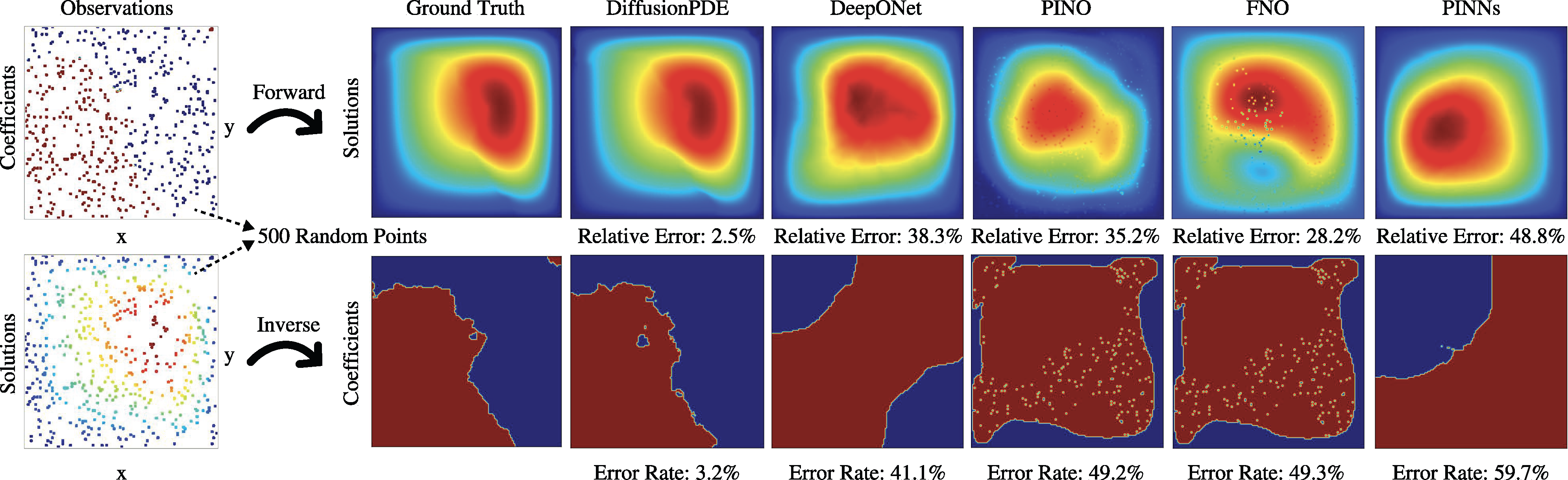
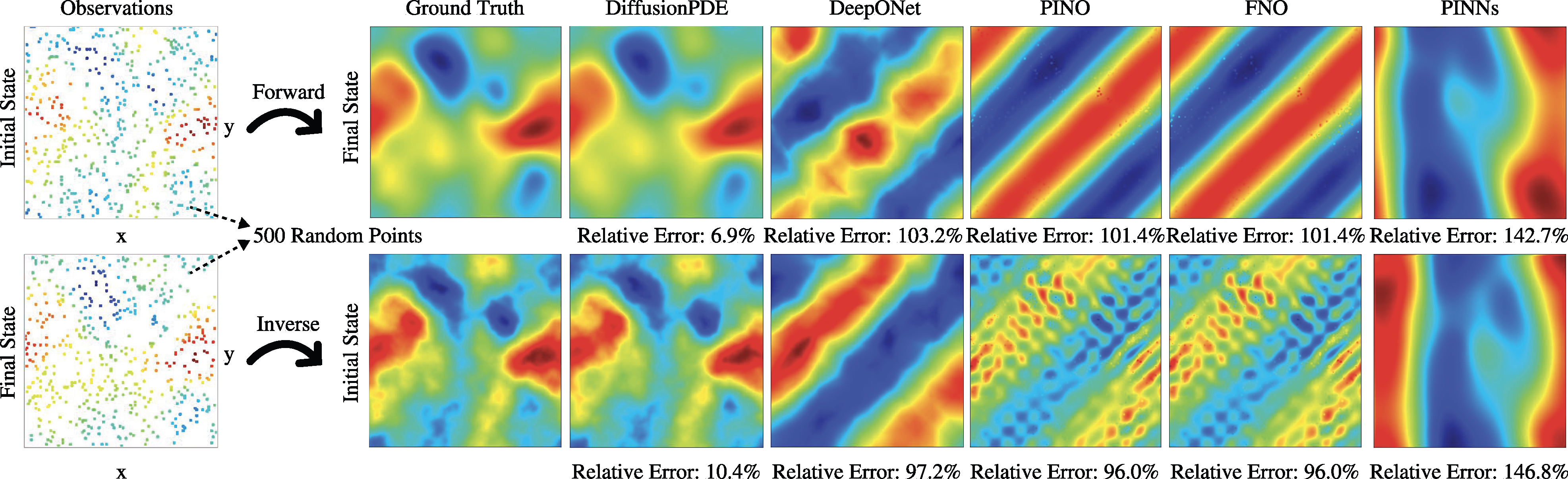
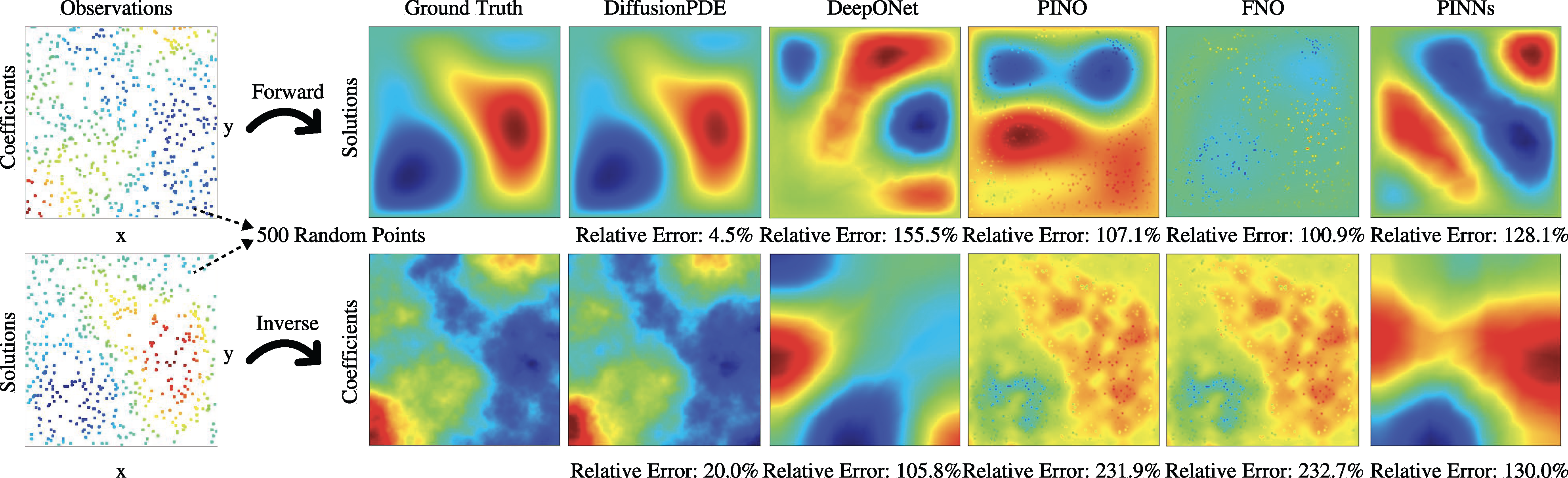
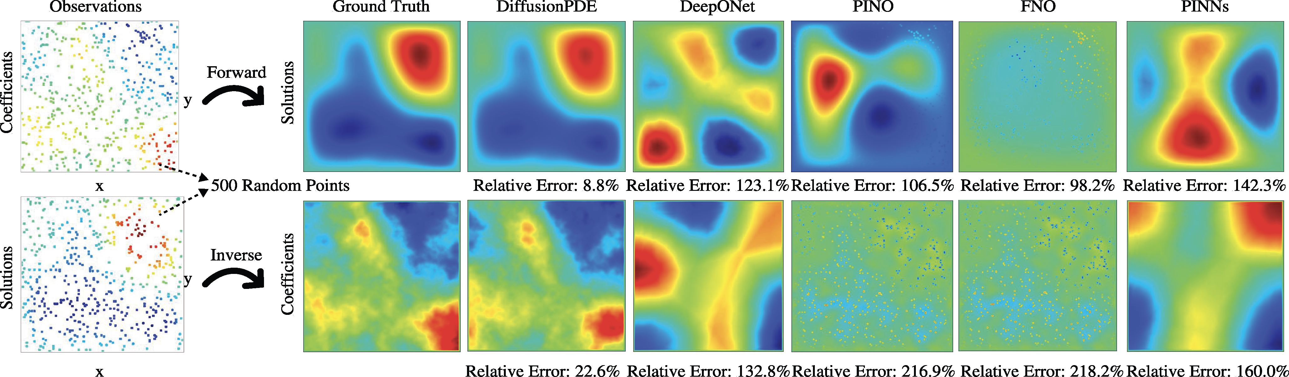
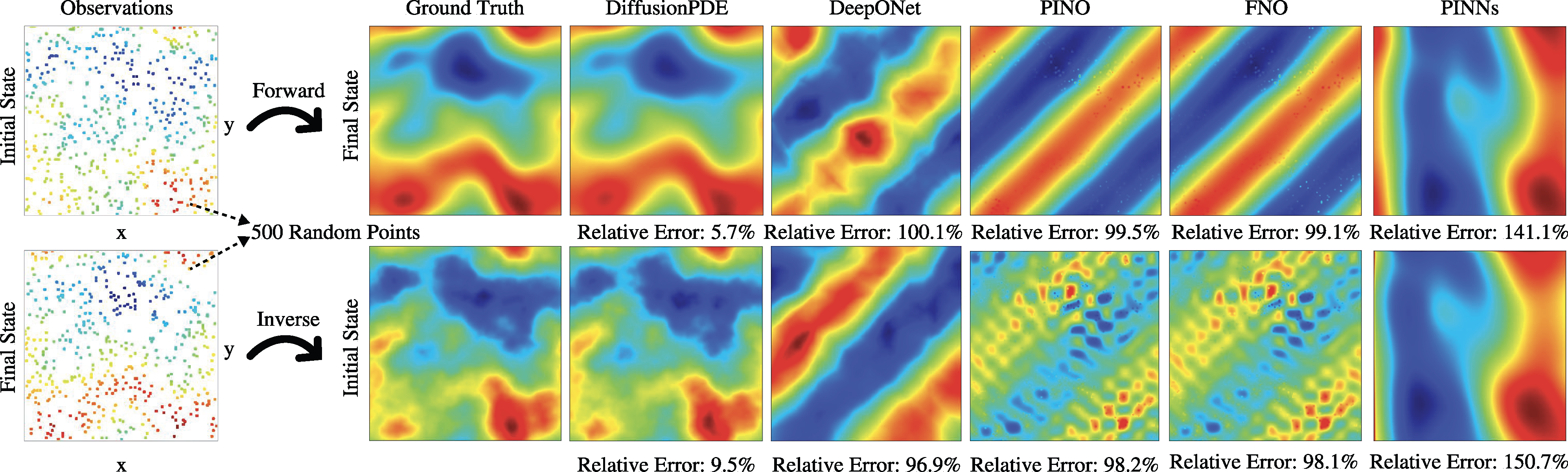
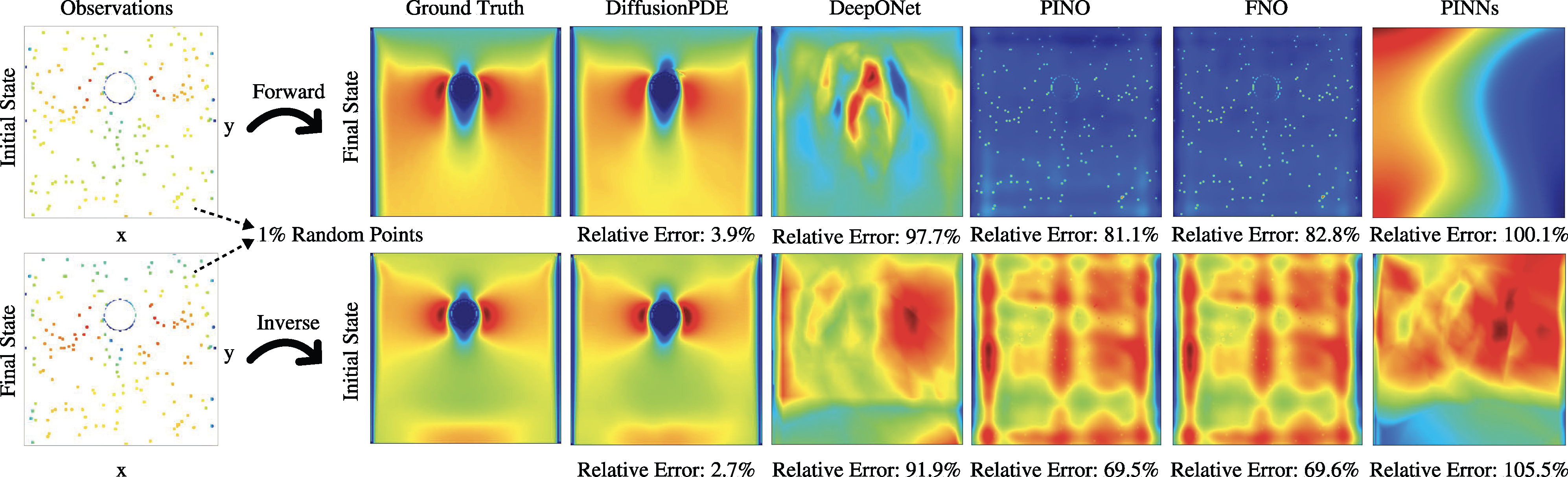
We address both forward and inverse problems of various types of PDEs with partial observations and compare the efficacy of our approach with state-of-the-art methods including DeepONet (Lu et al., 2021), PINO (Li et al., 2021), FNO (Li et al., 2020), and PINNs (Raissi et al., 2019). We show the relative errors of all methods regarding both forward and inverse problems with 500 observation points in Table 1. Since the coefficients of Darcy Flow are binary, we evaluate the error rates of our prediction. Non-binary data is evaluated using mean pixel-wise relative error. We report error numbers averaged across 1,000 random scenes and observations for each PDE. DiffusionPDE outperforms all other methods.

Table 1. Relative errors of solutions (or final states) and coefficients (or initial states) when solving forward and inverse problems with 500 observation points. Error rates are used for the inverse problem of Darcy Flow. Lower is better.
PDETaskDiffusionPDEPINODeepONetPINNsFNO
Darcy FlowForward2.5%35.2%38.3%48.8%28.2%
Inverse3.2%49.2%41.1%59.7%49.3%
PoissonForward4.5%107.1%155.5%128.1%100.9%
Inverse20.0%231.9%105.8%130.0%232.7%
HelmholtzForward8.8%106.5%123.1%142.3%98.2%
Inverse22.6%216.9%132.8%160.0%218.2%
Non-bounded Navier–StokesForward6.9%101.4%103.2%142.7%101.4%
Inverse10.4%96.0%97.2%146.8%96.0%
Bounded Navier–StokesForward3.9%81.1%97.7%100.1%82.8%
Inverse2.7%69.5%91.9%105.5%69.6%

Several examples of the forward and inverse problems are shown below.

Forward and inverse Darcy Flow results for all methods
Bounded Darcy Flow with 500 observation points of the coefficient or the solution.
Forward and inverse non-bounded Navier-Stokes results for all methods
Non-bounded Navier–Stokes equation for vorticity with 500 observation points of the initial state or the final state.
More results
Forward and inverse Poisson results for all methods
Bounded Poisson equation with 500 observation points of the coefficient or the solution.
Forward and inverse Helmholtz results for all methods
Bounded Helmholtz equation with 500 observation points of the coefficient or the solution.
Non-bounded Navier-Stokes results for all methods, another sample
Another sample of non-bounded Navier–Stokes equation for vorticity with 500 observation points of the initial state or the final state.
Bounded Navier-Stokes results for all methods
Bounded Navier–Stokes equation for velocity with a random circular obstacle and 1% observation points at the initial state or the final state.

Results

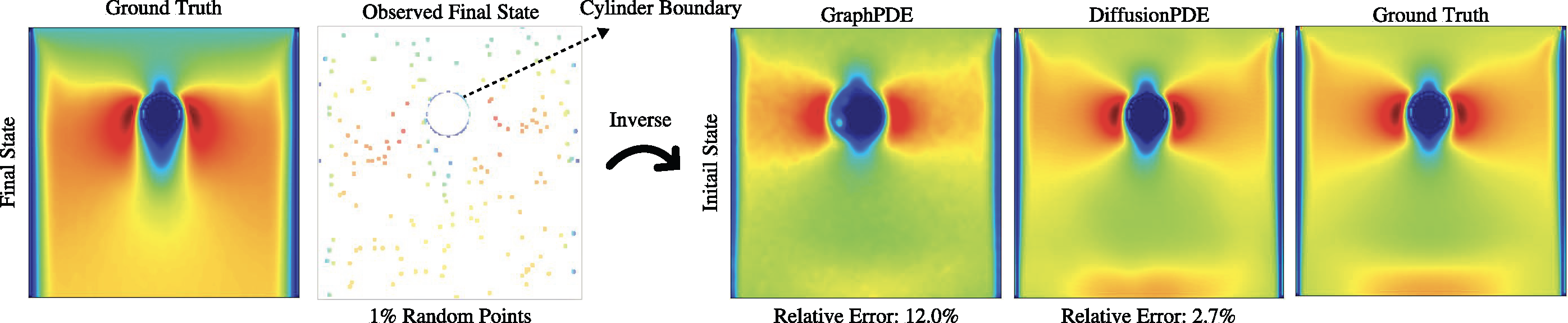
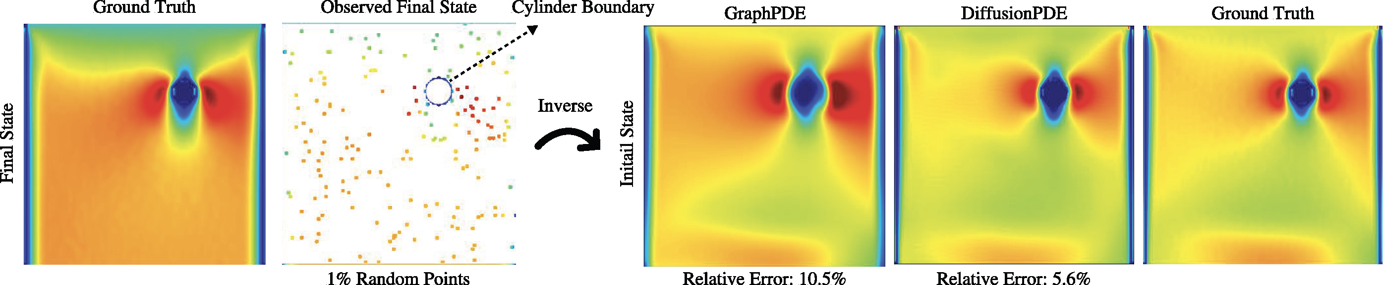
Comparisons with GraphPDE (Zhao et al., 2022)

Bounded Navier-Stokes inverse problem compared with GraphPDE, sample 1 Bounded Navier-Stokes inverse problem compared with GraphPDE, sample 2
Two samples of the inverse problem of bounded Navier–Stokes equation for velocity with a random circular obstacle and 1% observation points at the final state.

Results

Recovering Solutions Throughout a Time Interval

We retrieve all time steps throughout a time interval from continuous observations on sparse sensors.

Burgers' equation recovered over a time interval, sample 1 Burgers' equation recovered over a time interval, sample 2
Two samples of the Burgers’ equation with continuous observations from 5 out of 128 sensors.

BibTeX

@article{huang2024diffusionpde,
  title={DiffusionPDE: Generative PDE-solving under partial observation},
  author={Huang, Jiahe and Yang, Guandao and Wang, Zichen and Park, Jeong Joon},
  journal={Advances in Neural Information Processing Systems},
  volume={37},
  pages={130291--130323},
  year={2024}
}