TL;DR: RecFM is a new framework that aligns trajectories across scales for accurate generation, achieving one- and two-step generation for physics datasets comparable to state-of-the-art multi-step methods.
Ground Truth
RecFM (1-step)
VideoPDE
Channel 0
Ground Truth
RecFM (1-step)
VideoPDE
Channel 1
RecFM tracks the Helmholtz Staircase dynamics in one step, staying close to the ground-truth evolution across channels.
Abstract
Generative models have emerged as a powerful paradigm for solving physics systems and modeling complex spatiotemporal dynamics. However, achieving high physical accuracy without incurring high computational cost remains a fundamental challenge, as existing approaches face a critical speed-fidelity trade-off. In this work, we introduce Recursive Flow Matching (RecFM), a generative framework for forecasting complex spatiotemporal dynamics. RecFM enforces self-consistency to align trajectories across discretization scales, reducing discretization errors and improving performance across metrics for physics-based tasks. To our knowledge, this is the first method to achieve high-fidelity one- and few-step (2-4 step) dynamic generation for scientific systems with performance comparable to state-of-the-art multi-step solvers. Across challenging scientific benchmarks, RecFM achieves up to a 20× speedup over leading diffusion-based emulators while improving predictive accuracy. Furthermore, RecFM reduces mean squared error by over 15% compared to vanilla flow matching, offering a scalable and efficient solution for real-time scientific emulation.
Scientific Forecasting Results
Four-axis summary of the dynamic forecasting tasks. Metrics are averaged across datasets and normalized between [0, 1]; closer to 1 is better.
RecFM achieves strong forecasting performance across diverse scientific benchmarks, including Sea Surface Temperature (SST) forecasting, Navier-Stokes fluid dynamics, and the Helmholtz Staircase equation.
Compared to diffusion-based emulators such as VideoPDE (Li et al., 2025), RecFM substantially reduces rollout cost while improving predictive accuracy and physical consistency.
In particular, RecFM achieves up to 20× faster rollout generation than VideoPDE and over 15% lower MSE than vanilla Flow Matching while operating in the one- and few-step generation regime.
Quantitative forecasting results for Sea Surface Temperature, Navier-Stokes Flow, and Helmholtz Staircase Equation.
Lower values are better for MSE and CRPS, while the optimal SSR is 1.
Best results in bold, second best underlined, third best in gray.
Method
SST
Navier-Stokes
Helmholtz Staircase
CRPS
MSE
SSR
Time [s]
CRPS
MSE
SSR
CRPS
MSE
SSR
Perturbation*
0.281
0.180
0.411
0.4241
0.090
0.028
0.448
0.218
0.111
0.004
Dropout*
0.267
0.164
0.406
0.4241
0.078
0.027
0.715
0.099
0.049
0.631
DDPM*
0.246
0.177
0.674
0.3054
0.180
0.105
0.573
0.156
0.153
0.563
MCVD*
0.216
0.161
0.926
79.167
0.154
0.070
0.524
0.137
0.128
0.867
DYffusion*
0.224
0.173
1.033
4.6722
0.067
0.022
0.877
0.144
0.106
1.121
VideoPDE (Li et al., 2025)
0.216
0.162
0.746
19.753
0.033
0.0068
0.205
0.026
5.6e-4
4.334
Vanilla FM
0.260
0.232
0.914
1.5202
0.036
0.0076
0.911
0.030
6.5e-4
1.485
RecFM (1-step)
0.217
0.162
0.984
0.4310
0.031
0.0064
0.959
0.0034
4.2e-5
1.090
RecFM (2-step)
0.216
0.161
1.004
0.7353
0.032
0.0068
0.932
0.0027
2.7e-5
1.440
*Results for SST and Navier-Stokes are reproduced from DYffusion (Cachay et al., 2023).
Gallery
Navier-Stokes roll-out comparisons against FNO (Li et al., 2020) across velocity \(u\), velocity \(v\), and pressure \(p\):
Ground Truth
RecFM (1-step)
FNO
Velocity \(u\)
Ground Truth
RecFM (1-step)
FNO
Velocity \(v\)
Ground Truth
RecFM (1-step)
FNO
Pressure \(p\)
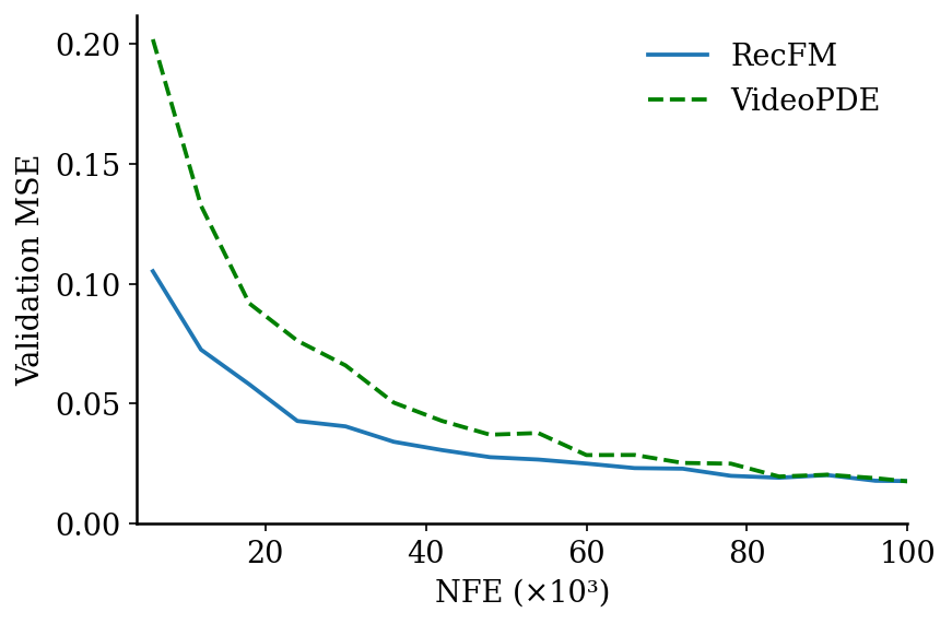
Training Stability
We compare training convergence on the Navier-Stokes benchmark
using cumulative function evaluations (NFE, i.e., number of forward passes) during optimization.
RecFM converges faster than the diffusion-based baseline
VideoPDE and consistently achieves lower validation error
throughout training.
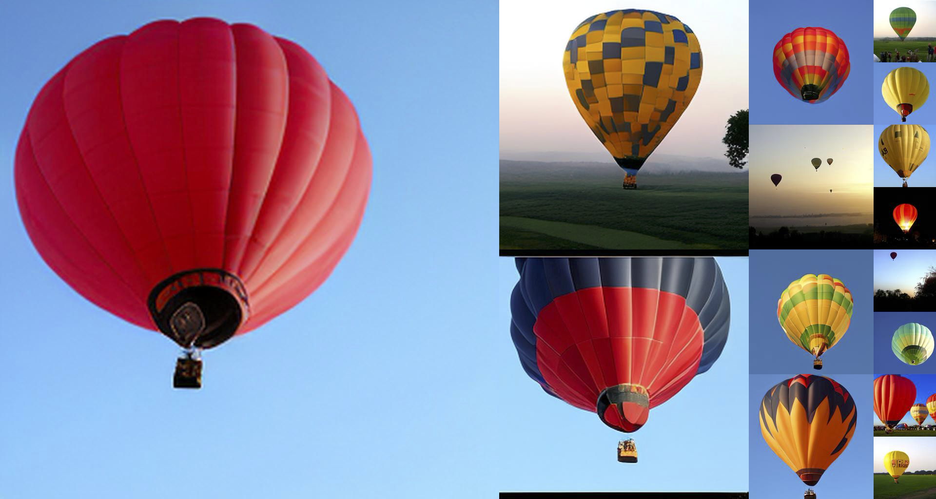
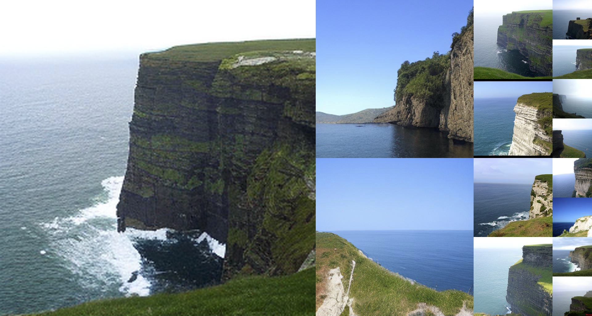
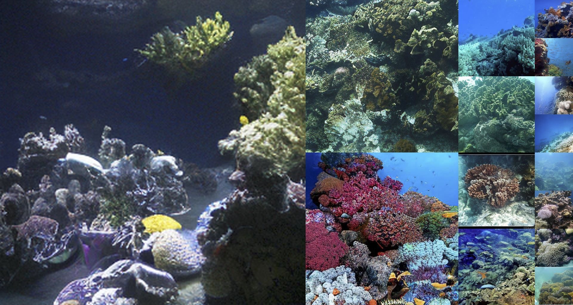
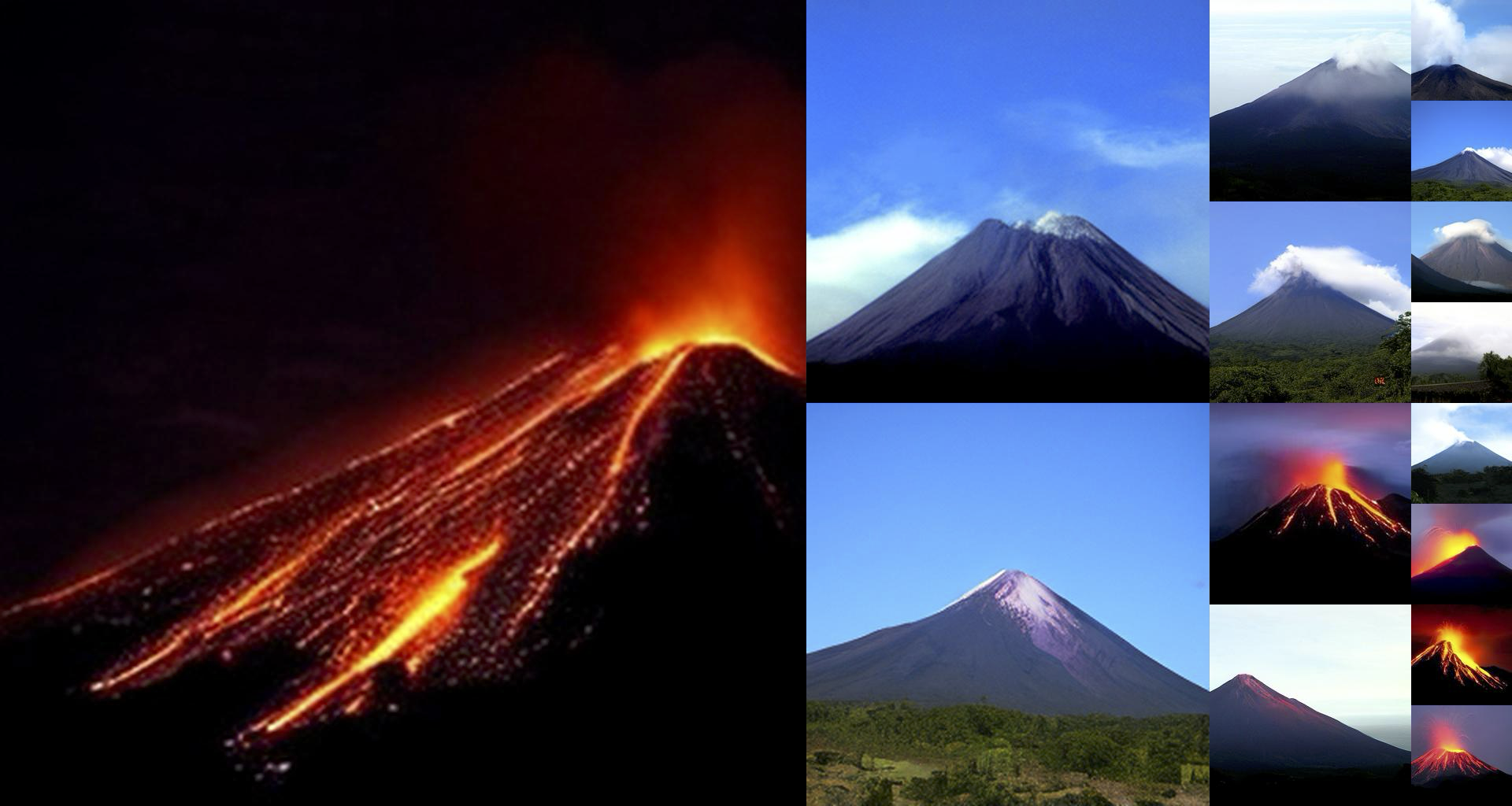
Image Generation Results
Shortcut Model
SiT
RecFM
t schedulert = 1.00
1.000.500.00
Denoising trajectories of Shortcut Model, SiT, and RecFM (8 inference steps).
We report results on ImageNet-1k dataset. RecFM is competitive in image generation as a multi-step flow matching method, while requiring fewer training epochs and inference steps.
Comparison of generative models under different sampling regimes.
Model
FID ↓
Sampling Steps
Param Count
Epochs Trained
DiT-XL (Peebles & Xie, 2023)
2.27
500
675M
640
SiT-XL (Ma et al., 2024)
2.06
250
675M
640
ADM-G (Dhariwal & Nichol, 2021)
4.59
250
—
426
LDM-4-G (Rombach et al., 2022)
3.6
500
400M
106
Shortcut Model (XL) (Frans et al., 2024)
3.8
128
676M
250
RecFM-XL
2.53
128
675M
160
RecFM-XL
2.49
16
675M
160
RecFM-XL
3.22
8
675M
160
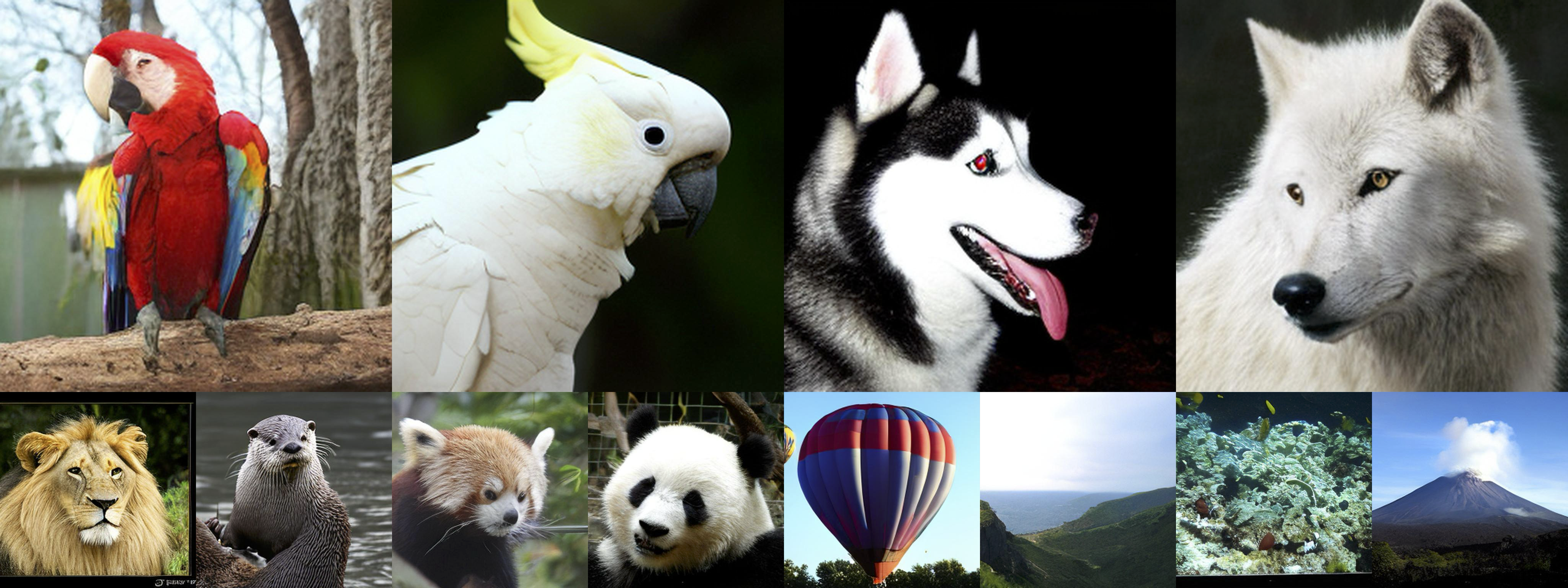
Below we visualize some image generation results for RecFM:
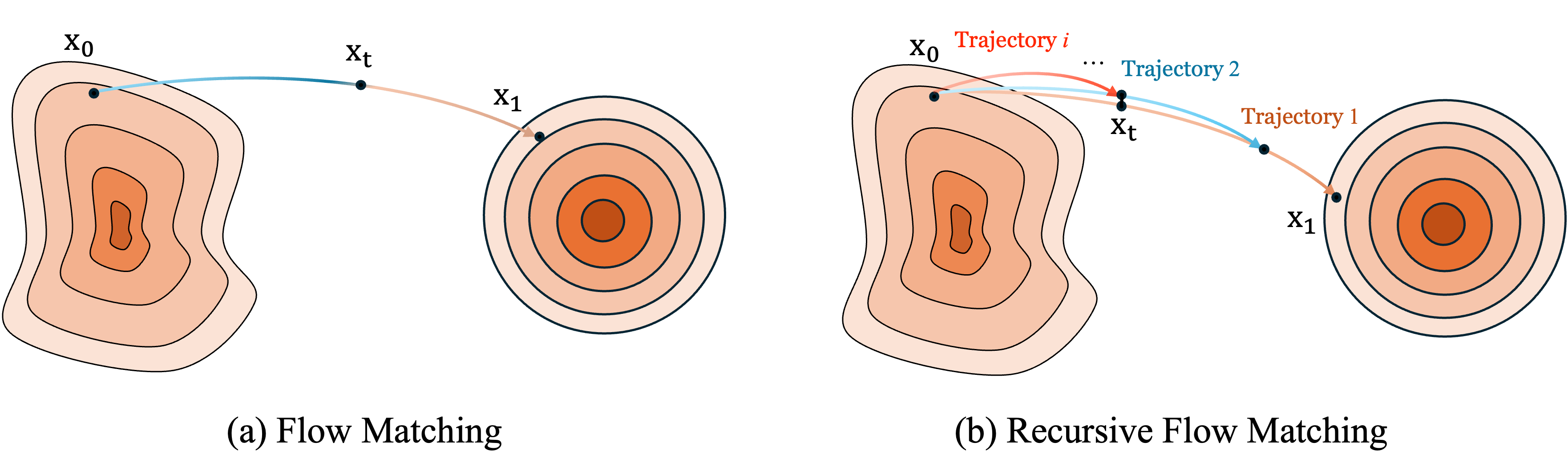
Standard Flow Matching learns a single trajectory between the data \(x_0\) and noise \(x_1\) distributions. RecFM instead models a family of recursively scaled trajectories that intersect at shared spatial states \(x_t\), enabling cross-scale consistency training and stable few-step generation.
Physics Intuition
Recursive Attenuation
After each collision, the pendulum loses energy and follows
a shorter trajectory with reduced velocity.
Trajectory Hierarchy
The recursive motion naturally produces a family of
progressively scaled trajectories that pass through the same point.
Connection to RecFM
RecFM enforces consistency by matching velocity predictions from
recursively scaled trajectories at the same spatial point.
Details
Recursive Flow Matching Formulation
Given a data sample \(x_0 \sim p_0\) and a noise sample
\(x_1 \sim p_1\), RecFM defines the standard linear interpolation
RecFM recursively constructs a family of trajectories across
different discretization scales. For recursion depth \(D\),
trajectories are parameterized by aligned time-scale pairs
\(\{(\tau^{(i)}, \alpha^{(i)})\}_{i=1}^{D}\), where
Under this alignment, all trajectories pass through the same
spatial state \(x_t\), leading to the recursive velocity relation
\[\hat{v}^{(i+1)} = \alpha \hat{v}^{(i)}.\]
RecFM trains a shared velocity network
\(v_\theta(x,\tau,\alpha)\) using multi-scale trajectory
supervision and cross-scale consistency constraints inspired by
the wall-bouncing pendulum dynamics.
Algorithm 1
Recursive Trajectory Training with Consistency Alignment
1
Require Data distribution \(p_0\), Noise distribution \(p_1\)
@misc{huang2026recursiveflowmatching,
    title={Recursive Flow Matching},
    author={Jiahe Huang and Sihan Xu and Sharvaree Vadgama and Rose Yu},
    year={2026},
    eprint={2605.26535},
    archivePrefix={arXiv},
    primaryClass={cs.LG},
    url={https://arxiv.org/abs/2605.26535},
}
References
Li, E., Wang, Z., Huang, J., & Park, J. J. (2025).
VideoPDE: Unified generative PDE solving via video inpainting diffusion models.
arXiv preprint arXiv:2506.13754.
Li, Z., Kovachki, N., Azizzadenesheli, K., Liu, B., Bhattacharya, K., Stuart, A., & Anandkumar, A. (2020).
Fourier neural operator for parametric partial differential equations.
arXiv preprint arXiv:2010.08895.
Frans, K., Hafner, D., Levine, S., & Abbeel, P. (2024).
One step diffusion via shortcut models.
arXiv preprint arXiv:2410.12557.
Rühling Cachay, S., Zhao, B., Joren, H., & Yu, R. (2023).
Dyffusion: A dynamics-informed diffusion model for spatiotemporal forecasting.
Advances in Neural Information Processing Systems, 36, 45259-45287.
Peebles, W., & Xie, S. (2023).
Scalable diffusion models with transformers.
Proceedings of the IEEE/CVF International Conference on Computer Vision, 4195-4205.
Dhariwal, P., & Nichol, A. (2021).
Diffusion models beat GANs on image synthesis.
Advances in Neural Information Processing Systems, 34, 8780-8794.
Rombach, R., Blattmann, A., Lorenz, D., Esser, P., & Ommer, B. (2022).
High-resolution image synthesis with latent diffusion models.
Proceedings of the IEEE/CVF Conference on Computer Vision and Pattern Recognition, 10684-10695.
Ma, N., Goldstein, M., Albergo, M. S., Boffi, N. M., Vanden-Eijnden, E., & Xie, S. (2024).
SiT: Exploring flow and diffusion-based generative models with scalable interpolant transformers.
European Conference on Computer Vision, 23-40.